Understanding Eigenvectors and Eigenvalues Visually

07-Jan-2015

Eigenvectors and eigenvalues are used in many engineering problems and have applications in object recognition, edge detection in diffusion MRI images, moments of inertia in motor calculations, bridge modelling, Google’s PageRank algorithm and more on wikipedia.

Previously, I wrote about visualising matrices and affine transformations. Here, we build on top of that and understand eigenvectors and eigenvalues visually.

Interpreting eigens

Quick recap, a non-zero matrix $x$ can be transformed by multiplying it with a $n \times n$ square matrix, $A$. So, the transformed matrix can be represented by the equation:
$$ T(x) = Ax $$

$x$ is called an eigenvector that when multiplied with $A$, yields a scalar value, $\lambda$, called the eigenvalue. The basic equation is:
$$ Ax = \lambda x $$

Any vector $v$ on the line made from the points passing through the origin $(0,0)$ and an eigenvector are all eigenvectors. Transforming $v$ by multiplying it by the transformation matrix $A$ or its associated eigenvalue $\lambda$ will result in the same vector. This will make more sense with the visuals in the following sections.

Most libraries (including numpy) will return eigenvectors that have been scaled to have a length of 1 (called unit vectors).

Eigenvalue $\lambda$ tells us how much $x$ is scaled, stretched, shrunk, reversed or untouched when multiplied by $A$. The number of eigenvalues is at most the number of dimensions, $n$. So, a set of 2D vectors will have at most 2 eigenvalues and corresponding eigenvectors.

Calculating eigenvalues, eigenvectors

Eigenvalue $\lambda$ and its corresponding eigenvector is found by solving the equation: $$det(\lambda I - A) = 0$$

What does determinant zero mean?
Heres a nice factsheet of determinant properties. If the $det(M) = 0$, $M$ is not invertible (columns cannot be swapped) and the rows and columns of $M$ are linearly dependent (one of the vectors in the set can be represented by the others. E.g {[2, 3], [4, 6]} are dependent as the second vector is a scaled version of the first vector in the set.)

You should watch Khan Academy’s example solving eigenvalues and the entire Eigen-eveything series if you want a step-by-step calculation and cement the maths. I also found these resources useful:

Eigens of a scaling transformation matrix

Lets start with a simple transformation matrix, $A = \begin{bmatrix}
2 & 0 \\
0 & 3
\end{bmatrix}$.


In [1]: A = np.matrix([[2, 0], [0, 3]])
In [2]: evals, evecs = np.linalg.eig(A)

Out[2]: evals:  [ 2.  3.]
        evecs: [[ 1.  0.]
                [ 0.  1.]]

The first eigenvalue, 2, is associated with the eigenvector in the first column (1, 0). Equation of the line through $(0,0)$ and $(1,0)$ is $y = 0$. So, any point on this line when multiplied by the transformation matrix $A$, will be scaled by 2.

Similarly, for the second eigenvalue, any point on the line $x = 0$ will be scaled by 3.

Visualising eigenvalues and eigenvectors

Lets use a more involved transformation matrix $A = \begin{bmatrix}
1 & 0.3 \\
0.45 & 1.2
\end{bmatrix}$.

For visualisation, we’ll plot a matrix $x = \begin{bmatrix}
-10 & -10 & 20 & 20\\
-10 & 20 & 20 & -10
\end{bmatrix}$ and its transformed state after it has been multiplied with $A$.

transformed_plot

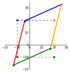
The dashed square shows the original matrix $x$ and the transformed matrix $Ax$. Now we’ll see where the eigens come into play.


In [1]: A = np.matrix([[1, 0.3], [0.45, 1.2]])
In [2]: evals, evecs = np.linalg.eig(A)

Out[2]: evals:  [ 0.71921134  1.48078866]
        evecs: [[-0.73009717 -0.52937334]
                 [ 0.68334334 -0.84838898]]

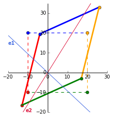
To plot the eigenvectors, we calculate the gradient:


In [1]: x_v1, y_v1 = evecs[:,0].getA1()
        x_v2, y_v2 = evecs[:,1].getA1()
In [2]: m1 = y_v1/x_v1 # Gradient of 1st eigenvector
        m2 = y_v2/x_v2 # Gradient of 2nd eigenvector

Out [2]: m1 = -0.936, m2 = 1.603  # Round to 3dp

So, our eigenvectors, which span all vectors along the line through the origin, have the equations: $y = -0.936x$ ($e1$) and $y = 1.603x$ ($e2$). This is plotted in blue and red below.

eigenvectors_plot

What does this eigen plot tell us?
The point where the first eigenvector line $e1$ intercepts the original matrix is $p1 = (10.68, -10)$. Multiplying this point by the corresponding eigenvalue of 0.719 OR by the transformation matrix $A$, yields $T(p1) = (7.684, -7.192)$.

$$ \begin{equation}
\begin{aligned}
A \times p1 \ &=
\begin{bmatrix}
1 & 0.3 \\
0.45 & 1.2
\end{bmatrix} & \times \begin{bmatrix}
10.68 \\
-10
\end{bmatrix} &= \begin{bmatrix}
7.684 \\
-7.192
\end{bmatrix} \\
\lambda \times p1 \ &=
0.719 & \times \begin{bmatrix}
10.68 \\
-10
\end{bmatrix} &=
\begin{bmatrix}
7.684 \\
-7.192
\end{bmatrix} \\
\end{aligned}
\end{equation} \\
\therefore Ax = \lambda x $$

Doing this for $e2$ will show the same calculation. As this eigenvector is associated with the largest eigenvalue of 1.481, this is the maximum possible stretch when acted by the transformation matrix.

To complete the visuals, we’ll plot $p1$ (the intercept with $e1$), $p2$ (the intercept with $e2$) and their transformed point $T(p1)$ and $T(p2)$.
Gist for the full plot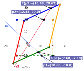
full_plot

Eigendecomposition

We can rearrange $Ax = \lambda x$ to represent $A$ as a product of its eigenvectors and eigenvalues by diagonalising the eigenvalues:
$$A = Q \Lambda Q^{-1}$$
with $Q$ as the eigenvectors and $\Lambda$ as the diagonalised eigenvalues. Using the values from the example above:

$$ \begin{bmatrix}
1 & 0.3 \\
0.45 & 1.2
\end{bmatrix} =
\begin{bmatrix}
-0.730 & -0.529 \\
0.683 & -0.848
\end{bmatrix}
\begin{bmatrix}
0.719 & 0 \\
0 & 1.481
\end{bmatrix}
\begin{bmatrix}
-0.730 & -0.529 \\
0.683 & -0.848
\end{bmatrix}^{-1} $$

To check this in Python:


In [1]: A = np.matrix([[1, 0.3], [0.45, 1.2]])
In [2]: evals, evecs = np.linalg.eig(A)
In [3]: np.allclose(A, evecs * np.diag(evals) * np.linalg.inv(evecs))
Out[3]: True

Next up, we’ll connect the eigen decomposition to another super useful technique, the singular value decomposition.

Alyssa Quek

data science