“The SVD is absolutely a high point of linear algebra” (Gilbert Strang, Kai Borre)
This mathematical technique has been used across various industries and example applications include recommender systems (Netflix prize), face and object recognition, risk modelling in equity options and identifying genes in brain imaging that make up Parkinson disease.
Definition
SVD is a matrix factorisation and decomposes a matrix of any size into a product of 3 matrices:
$$ A = U S V^T $$
$A$ : $n \times m$ : number of records as rows and number of dimensions/features as columns.
$U$ : $n \times n$ : orthogonal matrix containing eigenvectors of $AA^T$.
$S$ : $n \times m$ : ordered singular values in the diagonal. Square root of eigenvalues associated with $AA^T$ or $A^TA$ (its the same).
$V$ : $m \times m$ : orthogonal matrix containing eigenvectors of $A^TA$.
Orthogonal matrix: square matrix where columns make $90^\circ$ angles between each other and its inner dot product is zero. $Q^TQ = QQ^T = I$ and $Q^T=Q^{-1}$.
Orthonormal matrix: orthogonal matrix where columns are unit vectors.
Example matrix
For this post, Im going to use the same matrices from my post on eigenvectors and eigenvalues. We have a matrix $x = \begin{bmatrix}
-10 & -10 & 20 & 20\\
-10 & 20 & 20 & -10
\end{bmatrix}$ and a transformation matrix $A = \begin{bmatrix}
1 & 0.3 \\
0.45 & 1.2
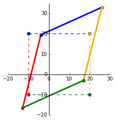
\end{bmatrix}$. In the plot below, the dashed square shows $x$ as the corners and the transformed matrix $Ax$ as the solid shape.

Python’s numpy provides us with a handy svd function:
In[1]:
A = np.matrix([[1, 0.3], [0.45, 1.2]])
U, s, V = np.linalg.svd(A)

Out[1]:
U:[[-0.58189652 -0.81326284]
   [-0.81326284  0.58189652]]
s:[ 1.49065822  0.71444949]
V:[[-0.63586997 -0.77179621]
   [-0.77179621  0.63586997]]
Lets verify some properties of the SVD matrices.
# Verify calculation of A=USV
In[2]:  np.allclose(A, U * np.diag(s) * V)
Out[2]: True

# Verify orthonormal properties of U and V. (Peformed on U but the same applies for V).
#  1) Dot product between columns = 0
In[3]:  np.round([np.dot(U[:, i-1].A1,  U[:, i].A1) for i in xrange(1, len(U))])
Out[3]: [ 0. 0.]

#  2) Columns are unit vectors (length = 1)
In[4]:  np.round(np.sum((U*U), 0))
Out[4]: [[ 1.  1.  1.]]

#  3) Multiplying by its transpose = identity matrix
In[5]:  np.allclose(U.T * U, np.identity(len(U)))
Out[5]: True
Geometric interpretation of SVD
Transformation of a matrix by $U S V^T$ can be visualised as a rotation and reflection, scaling, rotation and reflection. We’ll see this as a step-by-step visualisation.
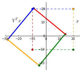
(1) $V^Tx$
We can see that multiplying by $V^T$ rotates and reflects the input matrix $x$. Notice the swap of colours red-blue and green-yellow indicating a reflection along the x-axis.
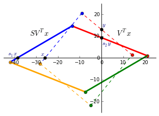
(2) $SV^Tx$
Since $S$ only contains values on the diagonal, it simply scales the matrix. The singular values $S$ are ordered in descending order so $s_1 > s_2 > … > s_n$. $V$ rotates the matrix to a position where the singular values now represent the scaling factor along the x and y-axis. This is now the V-basis.
The black dots shows this ($V^Tx$ is dashed and $SV^Tx$ solid):
- $V^Tx$ intercepts the x-axis at $x = -25.91$.
- Largest singular value of $s_1 = 1.49$ is applied and $s_1x = -38.61$.
- $V^Tx$ intercepts the y-axis at $y = 12.96$.
- Smallest singular value of $s_2 = 0.71$ is applied and $s_2y = 9.20$.

While not shown, there is a similar rotation and scaling effect in the U-basis with $Ux$ and $SUx$.
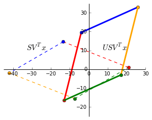
(3) $USV^Tx$
Finally, $U$ rotates and reflects the matrix back to the standard basis. As expected, this is exactly the same as $Ax$.

Eigen decomposition vs singular value decomposition
In an eigen-decomposition, $A$ can be represented by a product of its eigenvectors $Q$ and diagonalised eigenvalues $\Lambda$:
$$ A = Q \Lambda Q^{-1}$$.
- Unlike an eigen-decomposition where the matrix must be square ($n \times n$), SVD can decompose a matrix of any dimension.
- Column vectors in $Q$ are not always orthogonal so the change in basis is not a simple rotation. $U$ and $V$ are orthogonal and always represent rotations (and reflections).
- Singular values in $S$ are all real and non-negative. The eigenvalues in $\Lambda$ can be complex and have imaginary numbers.
Resources
SVD ties together the core concepts of linear algebra — matrix transformations, projections, subspaces, change of basis, eigens, symmetric matrices, orthogonalisation and factorisation. For a complete proof and backgound, I highly recommend the entire MIT Linear Algebra lectures by Gilbert Strang. I also found the examples and proofs for SVD and QR factorisation from the University of Texas’ MOOC useful.
Other posts covering SVD visualisations and its applications: