How do we find the major and minor axes of a blob?

We look at using 2 popular methods to obtain the same result:

1. Covariance matrix and eigenvectors, eigenvalues (partial PCA).
2. Raw image moments

1. Covariance matrix and eigens

An eigenvalue tells us the scaling magnitude along the direction of its corresponding eigenvector. Check my post on understanding eigens for the visual intuition.

Covariance matrix is a square and symmetric matrix that summarises the variance between two variables. So, with a set of $(x, y)$ points, the covariance matrix is 2x2:
$ C = \begin{bmatrix}
variance(x,x) & variance(x,y) \\
variance(x,y) & variance(y,y)
\end{bmatrix}$, where the variance of $(x, y)$ and $(y, x)$ are the same.

Principal component analysis (PCA) is a method commonly used for dimensionality reduction. The eigenvectors of the covariance matrix are called principal components. Heres a thorough tutorial on PCA and applied to computer vision (Lindsay Smith, 2002).

Eigenvectors with the largest eigenvalue of a covariance matrix gives us the direction along which the data has the largest variance.

Computation Outline

1. Matrix of points. We’ll be dealing with 2D points so our matrix is 2xm. The 1st row are the x-coordinates, 2nd row are the y-coordinates and m indicates the number of points.
2. Subtract the mean for each point. Calculate the mean of the row of x-coordinates. For each x-point, subtract the mean from it. Do the same for the y-coordinates. Mean subtraction minimises the mean square error of approximating the data and centers the data.
3. Covariance matrix calculation. Calculate the 2x2 covariance matrix.
4. Eigenvectors, eigenvalues of covariance matrix. Find the 2 eigen-pairs of our dataset.
5. Rearrange the eigen-pairs. Sort by decreasing eigenvalues.
6. Plot the principal components

Steps 1-5 are the beginning crux to performing dimensionality reduction with PCA.

Code Time

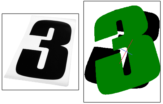
We’ll use a binary image as input and our matrix of points are the indices to the white pixels. Heres the image:

First, the libraries we’ll be using:

import numpy as np
import matplotlib.pyplot as plt
import scipy.misc
import skimage.filter

1) Read the image in grey-scale. We want the indexes of the white pixels to find the axes of the blob.

img = misc.imread('oval.png', flatten=1)
y, x = np.nonzero(img)

2) Subtract mean from each dimension. We now have our 2xm matrix.

x = x - np.mean(x)
y = y - np.mean(y)
coords = np.vstack([x, y])

3 & 4) Covariance matrix and its eigenvectors and eigenvalues

cov = np.cov(coords)
evals, evecs = np.linalg.eig(cov)

5) Sort eigenvalues in decreasing order (we only have 2 values)

sort_indices = np.argsort(evals)[::-1]
x_v1, y_v1 = evecs[:, sort_indices[0]]  # Eigenvector with largest eigenvalue
x_v2, y_v2 = evecs[:, sort_indices[1]]

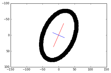
6) Plot the principal components. The larger eigenvector is plotted in red and drawn twice as long as the smaller eigenvector in blue.

scale = 20
plt.plot([x_v1*-scale*2, x_v1*scale*2],
         [y_v1*-scale*2, y_v1*scale*2], color='red')
plt.plot([x_v2*-scale, x_v2*scale],
         [y_v2*-scale, y_v2*scale], color='blue')
plt.plot(x, y, 'k.')
plt.axis('equal')
plt.gca().invert_yaxis()  # Match the image system with origin at top left
plt.show()

7) Bonus! We vertically-align the blob based on the major axis via a linear transformation. An anti-clockwise rotating transformation matrix has the general form: $\begin{bmatrix}
cos \theta & -sin \theta \\
sin \theta & cos \theta
\end{bmatrix}$.

To do this:

1. Calculate $\theta$ using the eigenvector of the major axis to the y-axis
2. Create the rotating transformation matrix
3. Multiply the transformation matrix to the set of coordinates.

   
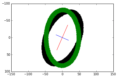
   theta = np.arctan((x_v1)/(y_v1))  
   rotation_mat = np.matrix([[np.cos(theta), -np.sin(theta)],
                         [np.sin(theta), np.cos(theta)]])
   transformed_mat = rotation_mat * coords
   # plot the transformed blob
   x_transformed, y_transformed = transformed_mat.A
   plt.plot(x_transformed, y_transformed, 'g.')
   

The vertically-align transformed blob is overlaid in green.

2. Raw image moments

We can obtain the same axes and orientation of a blob with raw image moments and central moments. Special thanks to this stack overflow answer.

The calculation of a raw image moment is given by the equation:

\begin{aligned}
M_{ij} = \sum\limits_{y=0}^{nrows}\sum\limits_{x=0}^{ncols} x^i \ y^j \ I(x, y)
\end{aligned}

where $x$ and $y$ are indices to the data and $I(x, y)$ is the grey-level intensity value at that index. The codification of that equation:

def raw_moment(data, i_order, j_order):
  nrows, ncols = data.shape
  y_indices, x_indicies = np.mgrid[:nrows, :ncols]
  return (data * x_indicies**i_order * y_indices**j_order).sum()

Now we can derive the second order central moments and construct its covariance matrix:

def moments_cov(data):
  data_sum = data.sum()
  m10 = raw_moment(data, 1, 0)
  m01 = raw_moment(data, 0, 1)
  x_centroid = m10 / data_sum
  y_centroid = m01 / data_sum
  u11 = (raw_moment(data, 1, 1) - x_centroid * m01) / data_sum
  u20 = (raw_moment(data, 2, 0) - x_centroid * m10) / data_sum
  u02 = (raw_moment(data, 0, 2) - y_centroid * m01) / data_sum
  cov = np.array([[u20, u11], [u11, u02]])
  return cov

Note that calculating the image moments does not require finding the indices to the blob shape. To use the above function, simply call it with the image data:

img = misc.imread('oval.png', flatten=1)
cov = moments_cov(img)
evals, evecs = np.linalg.eig(cov)

Given the covariance matrix, finding the axes and re-aligning the blob continues with steps 4 to 7 from the first method. As expected, the transformed plot looks the same:

Comparison

In this case, using image moments would be faster since we do not have to find the $(x, y)$ coordinates to the blob pixels. Both methods would encounter issues with images containing lots of noise.

The partial PCA calculated the largest eigenvalue of 2942.0060 and its eigenvector [0.3997, -0.9166]. By a slight difference, image moments returned the largest eigenvalue of 2943.2583 and its eigenvector of [0.4027, -0.9153].
Their $\theta$ difference is less than a fifth of $1^\circ$.

For asymmetric blobs, both methods will be biased to the side that has the higher concentration of pixels. Heres an image where the axes appear to be slightly off and over-rotates in an attempt to align it (original image on the left):