The Hough transform (Duda and Hart, 1972), which started out as a technique to detect lines in an image, has been generalised and extended to detect curves in 2D and 3D.
Here, we understand how an image is transformed into the hough space for line detection and implement it in Python.
How it works - gradient-intercept parameter space
A line in Cartesian form has the equation: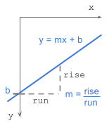
y = mx + b

where:
m = gradient or slope of the line (rise/run)
b = y-intercept
Given a set of edge points or a binary image indicating edges, we want to find as many lines that connect these points in image space.
Say we have 2 edge points ($x_1, y_1$) and ($x_2, y_2$). For each edge point at various gradient values ($m$=-0.5, 1.0, 1.5, etc), we calculate the corresponding $b$ values. The image below shows the various lines through an edge point in image space and the plot of these lines in parameter space. Points which are collinear in the cartesian image space will intersect at a point in $m$-$b$ parameter space.
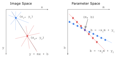
All points on a line in image space intersect at a common point in parameter space. This common point ($m$, $b$) represents the line in image space.
Unfortunately, the slope, $m$, is undefined when the line is vertical (division by 0!).
To overcome this, we use another parameter space, the hough space.
How it works - angle-distance parameter space
A line in Polar coordinate system has the equation:
ρ = x cos θ + y sin θ

where:
ρ (rho) = distance from origin to the line. [-max_dist to max_dist].
          max_dist is the diagonal length of the image.
θ = angle from origin to the line. [-90° to 90°]
If you’re interested in how $\rho$ is derived, I’ve laid out the maths at the bottom extras section: deriving rho.
To explain the hough transform, I’ll use a simple example. I’ve created an input binary image of size 30 x 30 pixels with points at (5, 25) and (20, 10) shown below. The image is transformed to the hough space by calculating $\rho$ with a point at each angle from $-90^\circ$ to $90^\circ$ (negative angles are anti-clockwise starting horizontally from the origin and positive angles are clockwise). The points in hough space make a sinusoidal curve.
![]()
The value of $\rho$ at various angles for the 2 edge points:
| point | $-90^\circ$ | $-45^\circ$ | $0^\circ$ | $45^\circ$ | $90^\circ$ |
|---|---|---|---|---|---|
| (5, 25) | -25 | -14 | 5 | 21 | 25 |
| (20, 10) | -10 | 7 | 20 | 21 | 10 |
![]()
We see that the curves in hough space intersect at $45^\circ$ with $\rho=21$.
Curves generated by collinear points in the image space intersect in peaks $(\rho, \theta)$ in the Hough transform space. The more curves intersect at a point, the more “votes” a line in image space will receive. We’ll see this in the next implementation section.
Algorithm steps
- Corner or edge detection. (E.g. using canny, sobel, adaptive thresholding). The resultant binary/grey image will have 0s indicating non-edges and 1s or above indicating edges. This is our input image.
- Rho range and Theta range creation. $\rho$ ranges from -max_dist to max_dist where max_dist is the diagonal length of the input image. $\theta$ ranges from $-90^\circ$ to $90^\circ$. You can have more or less bins in the ranges to tradeoff accuracy, space and speed. E.g. Every third angle in $-90^\circ$ to $90^\circ$ to reduce from 180 to 60 values.
- Hough accumulator of $\theta$ vs $\rho$. It is a 2D array with the number of rows equal to the number of $\rho$ values and the number of columns equal to the number of $\theta$ values.
- Voting in the accumulator. For each edge point and for each $\theta$ value, find the nearest $\rho$ value and increment that index in the accumulator. Each element tells how many points/pixels contributed “votes” for potential line candidates with parameters $(\rho, \theta)$.
- Peak finding. Local maxima in the accumulator indicates the parameters of the most prominent lines in the input image. Peaks can be found most easily by applying a threshold or a relative threshold (values equal to or greater than some fixed percentage of the global maximum value).
Code Time
Full code on github
import numpy as np

def hough_line(img):
  # Rho and Theta ranges
  thetas = np.deg2rad(np.arange(-90.0, 90.0))
  width, height = img.shape
  diag_len = np.ceil(np.sqrt(width * width + height * height))   # max_dist
  rhos = np.linspace(-diag_len, diag_len, diag_len * 2.0)

  # Cache some resuable values
  cos_t = np.cos(thetas)
  sin_t = np.sin(thetas)
  num_thetas = len(thetas)

  # Hough accumulator array of theta vs rho
  accumulator = np.zeros((2 * diag_len, num_thetas), dtype=np.uint64)
  y_idxs, x_idxs = np.nonzero(img)  # (row, col) indexes to edges

  # Vote in the hough accumulator
  for i in range(len(x_idxs)):
    x = x_idxs[i]
    y = y_idxs[i]

    for t_idx in range(num_thetas):
      # Calculate rho. diag_len is added for a positive index
      rho = round(x * cos_t[t_idx] + y * sin_t[t_idx]) + diag_len
      accumulator[rho, t_idx] += 1

  return accumulator, thetas, rhos
Usage:
# Create binary image and call hough_line
image = np.zeros((50,50))
image[10:40, 10:40] = np.eye(30)
accumulator, thetas, rhos = hough_line(image)

# Easiest peak finding based on max votes
idx = np.argmax(accumulator)
rho = rhos[idx / accumulator.shape[1]]
theta = thetas[idx % accumulator.shape[1]]
print "rho={0:.2f}, theta={1:.0f}".format(rho, np.rad2deg(theta))
rho=0.50, theta=-45
Hough transform (and the faster probabilistic version) is available in openCV and scikit-image.
Extensions
Hough transform can be extended to detect circles of the equation
$r^2 = (x − a)^2 + (y − b)^2$ in the parameter space, $\rho = (a, b, r)$.
Furthermore, it can be generalized to detect arbitrary shapes (D. H. Ballard, 1981).
Another approach is the Progressive Probabilistic Hough Transform (Galamhos et al, 1999). The algorithm uses random subsets of voting points in the accumulator and checks for the longest segment of pixels with minimum gaps. Line segments that exceed a minimum length threshold are added to the list. This returns the beginning and end point of each line segment in the image. It has 3 thresholds: a minimum number of votes in the Hough accumulator, a maximum line gap for merging and a minimum line length.
Extras
Deriving rho: ρ = x cos θ + y sin θ
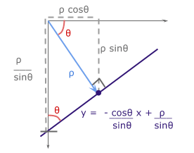
With basic trigonometry, we know that for right-angled triangles,
$sin \theta = {opposite\over hypotenuse}$ and $cos \theta = {adjacent \over hypotenuse}$.
We want to convert the cartesian form $y = mx + b$ with parameters $(m, b)$ to polar form with parameters $(\rho, \theta)$.
The line from the origin with distance $\rho$ has a gradient of ${sin \theta \over cos \theta}$. The line of interest, which is perpendicular to it, will have a negative reciprocal gradient value of ${-cos \theta \over sin \theta}$. For $b$, the y-intercept of the line of interest, $sin \theta = {\rho \over b}$.
With $m = {-cos \theta \over sin \theta}$ and $b = {\rho \over sin \theta}$, we get $\rho = x \ cos \theta + y \ sin \theta$.